COMP305
COMP305 W1-6
introduction
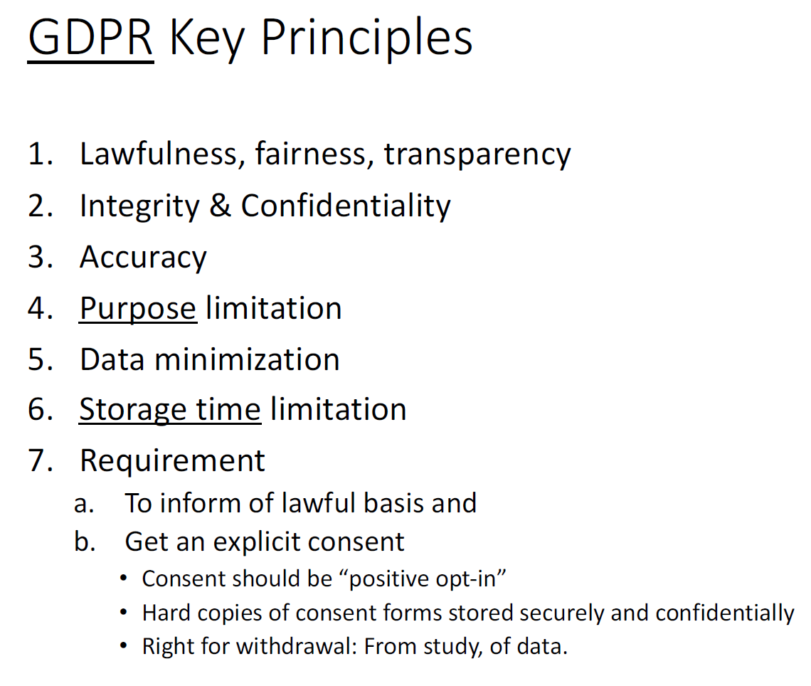
- Lawfulness, fairness, transparency 透明度
- Integrity & Confidentiality
- Accuracy
- Purpose limitation
- Data minimization
- Storage time limitation
- Requirement
ANN
propagation 传播
spikes 峰值
threshold 阈值
intensity 强度
duration 持续时间
……
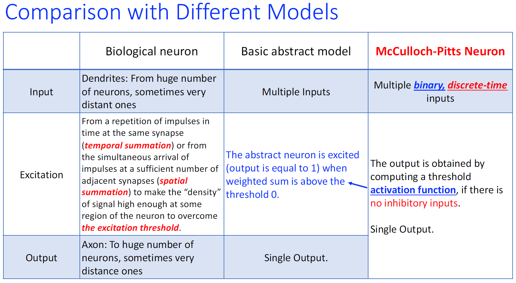
Discrete Time + Binary Input
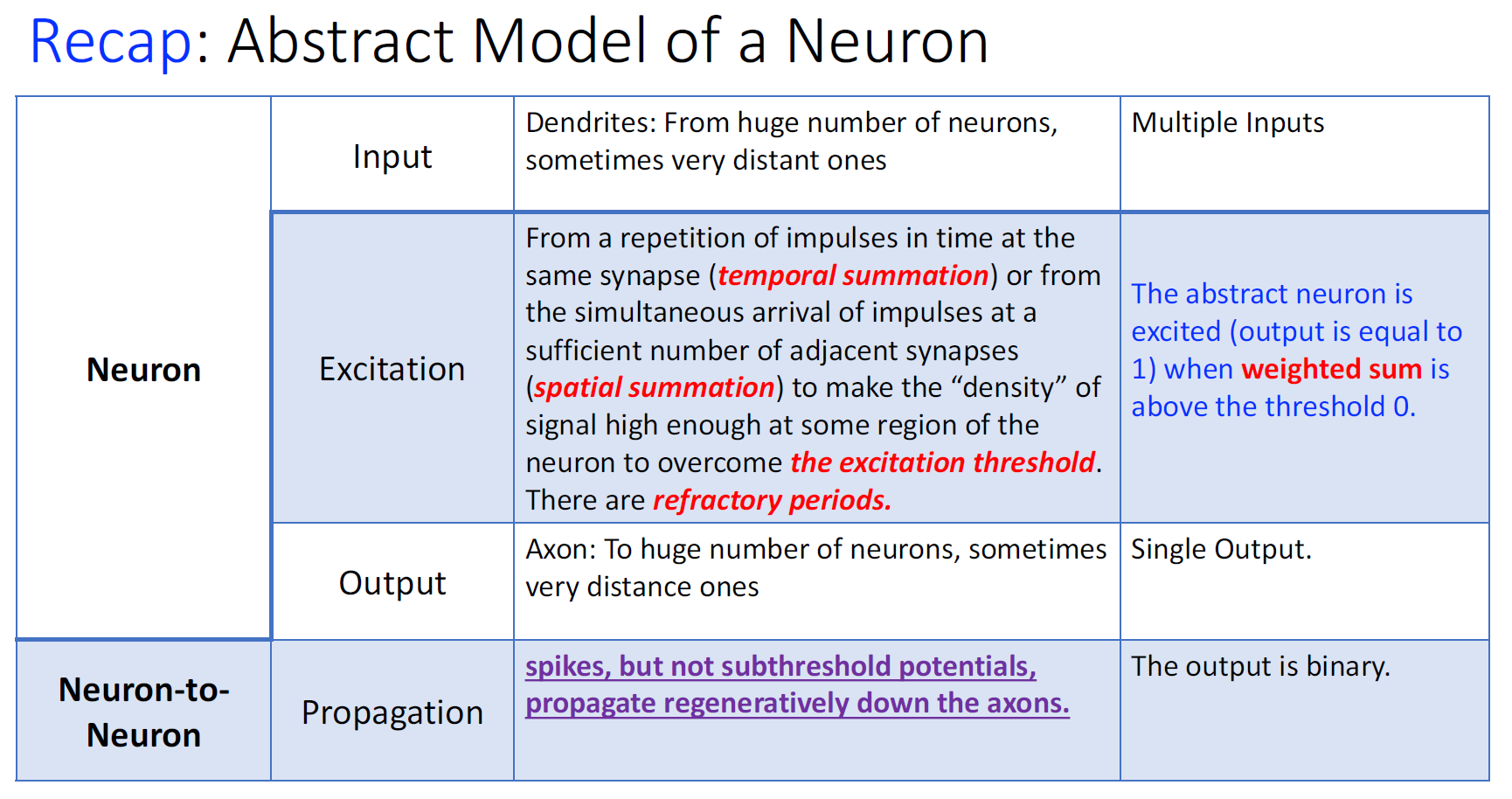
密度够高:temporal summation > excitation threshold
输入够多:spatial summation > excitation threshold
refractory period:不应期 ---> Discrete Time
in/output unified
McCulloch-Pitts Neuron
excitatory connection:+1 兴奋/激活连接
inhibitory connection: -1 抑制连接
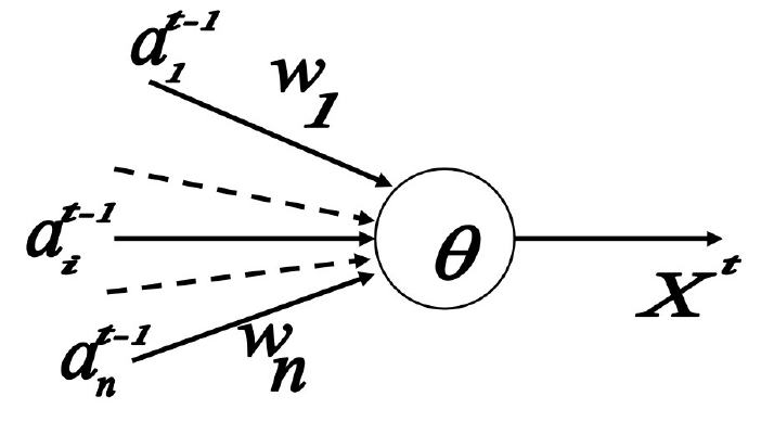 \[
X^t=1 \text { if and only if } S^{t-1}=\sum w_i a_i^{t-1} \geq \theta
\text {, and } w_i>0, \forall a_i^{t-1}>0
\] 说白了就是 no inhibitory connection is
activited and sum is larger than threshold.
\[
X^t=1 \text { if and only if } S^{t-1}=\sum w_i a_i^{t-1} \geq \theta
\text {, and } w_i>0, \forall a_i^{t-1}>0
\] 说白了就是 no inhibitory connection is
activited and sum is larger than threshold.
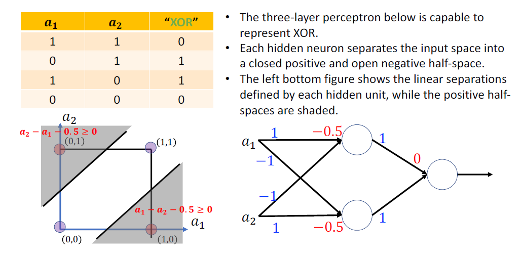
What can we do with a MP neuron?
Simple logical functions: AND, OR and NOT
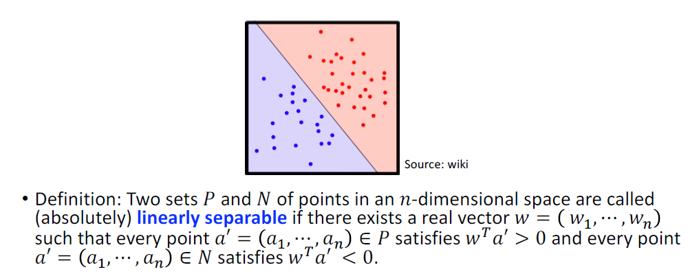
必须是 Linear separable 的
完备性?:

形式化,等价图灵机
An MP neural network can implement any multivariable propositional logic function, with the thresholds and weights being appropriately selected.
Furthermore, the discrete time, or unity delay property of the model makes it even possible to build a sequential digital circuitry.
Hebb’s Rule
The simplest formulation of Hebb’s rule is to increase weight of connection at every next instant in the way
\[ w_i^{t+1}=w_i^t+\Delta w_i^t, \] Where \[ \Delta w_i^t=C a_i^t X^{t+1} \] | | | | -------------- | ----------------------------------------------------------- | | \(w_i^{t}\) | the weight of connection at instant \(t\) | | \(w_i^{t+1}\) | the weight of connection at the next instant \(t+1\) | | \(\Delta w_i^t\) | the increment by which the weight of connection is enlarged | | \(C\) | positive coefficient which determines learning rate | | \(a_i^t\) | input value from the presynaptic neuron at instant | | \(X^{t+1}\) | output of the postsynaptic neuron at the instant \(t+1\) |
Algorithm of Hebb’s Rule for a Single Neuron (NOT MP)
- Set the neuron threshold value \(\theta\) and the learning rate \(C\).
- Set random initial values for the weights of connections \(w_i^t\).
- Give instant input values \(a_i^t\) by the input units.
- Compute the instant state of the neuron \(S^t=\sum_i w_i^t a_i^t\)
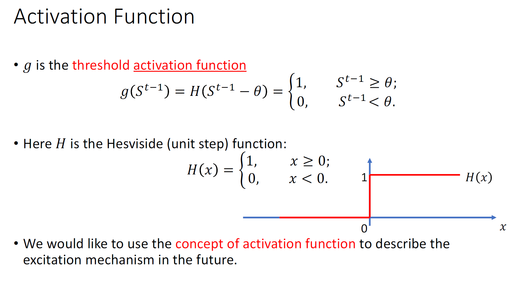
- Compute the instant output of the neuron \(X^{t+1}\) \[ X^{t+1}=g\left(S^t\right)=H\left(S^t-\theta\right)= \begin{cases}1, & S^t \geq \theta \\ 0, & S^t<\theta\end{cases} \]
- Compute the instant corrections to the weights of connections \(\Delta w_i^t=\) \(C a_i^t X^{t+1}\)
- Update the weights of connections \(w_i^{t+1}=w_i^t+\Delta w_i^t\)
- Go to the step 3.
Normalized Hebb’s Rule (Oja’s Rule)
Formulation of Normalized Hebb’s Rule (Oja’s rule)
- Set the neuron threshold value \(\theta\) and the learning rate \(C\).
- Set random initial values for the weights of connections \(w_i^t\).
- Normalization.
- Give instant input values \(a_i^t\) by the input units.
- Compute the instant state of the neuron \(S^t=\sum_i w_i^t a_i^t\)
- Compute the instant output of the neuron \(X^{t+1}\)
\[ X^{t+1}=g\left(S^t\right)=H\left(S^t-\theta\right)= \begin{cases}1, & S^t \geq \theta \\ 0, & S^t<\theta\end{cases} \]
- Compute the instant corrections to the weights of connections \(\Delta w_i^t=\) \(C a_i^t X^{t+1}\)
- Update the weights of connections \(w_i^{t+1}=w_i^t+\Delta w_i^t\)
- Go to the step 3.
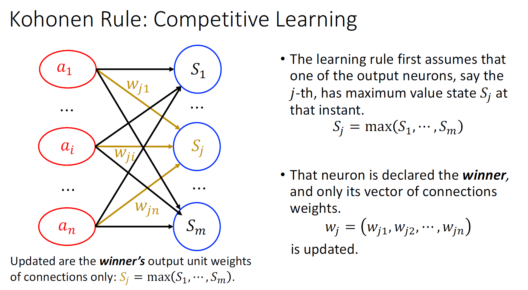
Kohonen’s Rule (Competitive Learning)
Hebb’s Rule+ winner takes it all
Unsupervised Learning Unsupervised learning is a type of machine learning in which the algorithm is not provided with any pre-assigned labels or scores for the training data. As a result, unsupervised learning algorithms must first self-discover any naturally occurring patterns in that training data set.
A common example is clustering (聚类), that is, an unsupervised network can group similar sets of input patterns into clusters predicated upon a predetermined set of criteria relating the components of the data.
Clustering can be achieved when we extend the single neuron to the network with multiple outputs.
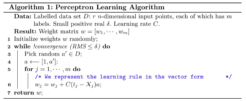
Perceptron
A Perceptron is a neural network that changes with “experience” using an error-correction rule
• Training set: a set of input patterns repeatedly presented to the network during training; • Target output (label): the predefined correct output of an input pattern in the training set.
According to the rule, weight of a response unit changes when it makes error response to the input presented to the network.
The network outputs 𝑿𝒋 are then compared to the desired outputs specified in the training set and obtain the error.
SUM OF INPUT * WEIGHT \[ S_j=\sum_{i=0}^n w_{j i} a_i \] \[ X_j=f(S_j) \] \[ e_j=(t_j-X_j) \]
\[ \begin{gathered} \Delta w_{j i}^k=C e_j^k a_i^k\\ \\ w_{j i}^k=w_{j i}^k+\Delta w_{j i}^k \end{gathered} \]
对于多输出, The network performance during training session is measured by a root-mean-square (RMS) error value : \[ \mathrm{RMS}=\sqrt{\frac{\sum_{k=1}^r \sum_{j=1}^m\left(e_j^k\right)^2}{r m}} \]
对于\(w^k_{ji}\) k是所在元层数,j是指向元编号,i是本元编号。
The process of weights adjustment is called perceptron “learning” or “training”.
fully interconnected:every input neuron is connected to every output neuron.
Single Perceptron's output is binary
L15 2p 过程
L16
Convergence of Perceptron Learning Algorithm
Hidden Neurons
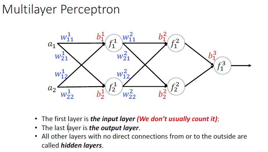
• The input is processed and propagated from one layer to the next, until the final result is computed. • This process represents the forward propagation.
L18
The output error of a multilayer perceptron for the 𝑘-th input pattern is a half of the squared error: \[ E^k=\frac{1}{2} \sum_{j=1}^m\left(e_j^k\right)^2=\frac{1}{2} \sum_{j=1}^m\left(t_j^k-X_j^k\right)^2 \] error backpropagation 要用梯度下降法Gradient descent
对于梯度下降法,我们需要使用generic sigmoidal activation function以作激活函数 activation function: \[ f(S)=\frac{\alpha}{1+e^{-\beta S+\gamma}}+\lambda \] 那么,我们就有导数: \[ f^{\prime}(S)=\frac{d f}{d S}=\frac{\beta}{\alpha} \cdot(f(S)+\lambda)(\alpha+\lambda-f(S)) \]
然后change weight \[ w_{j i}^k=w_{j i}^k+\Delta w_{j i}^k\\ \Delta w_{j i}^k =-C \frac{\partial E}{\partial w_{j i}^k} \]
Genetic Algorithms
L21
生物
crossing-over
Mutation is a random change of a “letter”, single nucleotide in a chromosome.
Different possible settings for a trait, e.g. blue, brown, black eye colour, are called alleles.
The complete collection of all genetic material, that is all chromosomes taken together, is called the organism’s genome or genotype.
L22
自然演化:
Parallelism:Every individual in the population is tested independently in parallel with the others, and that speeds up evolution of the population.
Adaptation:Due to the natural selection, only those individuals best fitted for the current environment do survive. The selection results in the population as a whole best adapted to the environment.
Optimization:Due to the natural selection, only individuals best fitted or “optimal” for the current environment do survive and reproduce. Thus, the selection also performs optimization on an individual level.
L23
GAs by John Holland.
Holland introduced • a “population” of binary strings (a string of characters) which he called “chromosomes”. • The “population” evolves using kind of “natural selection” together with the genetics-inspired operators of crossover, mutation, and inversion. • Bits in a “chromosome” represent genes, and each “gene” is an instance of a particular “allele”, 0 or 1.
• The selection operator chooses those chromosomes in the population that will be allowed to reproduce, and on average the fitter chromosomes produce more offspring than the less fit ones. • Crossover exchange subparts of two chromosomes • Mutation randomly changes the allele values at some locations in the chromosome. • Inversion reverses the order of a continuous section of the chromosome rearranging the genes order.
• *Translocation is a mutation when part of a chromosome is cut out and moved to a different location in the chromosome.
Population of chromosomes is the evolving unit 进化的单位
Fitness Function
To evaluate how good the candidate solution solves the problem
• Takes a chromosome as an input; • Produces its quantitative fitness evaluation as an output.
Two important requirements: • Should correlate closely with the designer's goal • Should be computationally efficient
Search Space:Set of all possible solutions to a problem in consideration is called a Genetic Algorithm search space.
Fitness Landscape:representation of all possible solutions along with their fitness.
L24
Basic Structure of a Genetic Algorithm
- Randomly generate initial population of n bit strings (“chromosomes”).
- Evaluate the fitness of each string in the population.
- Repeat the following steps until next generation of n individual
produced.
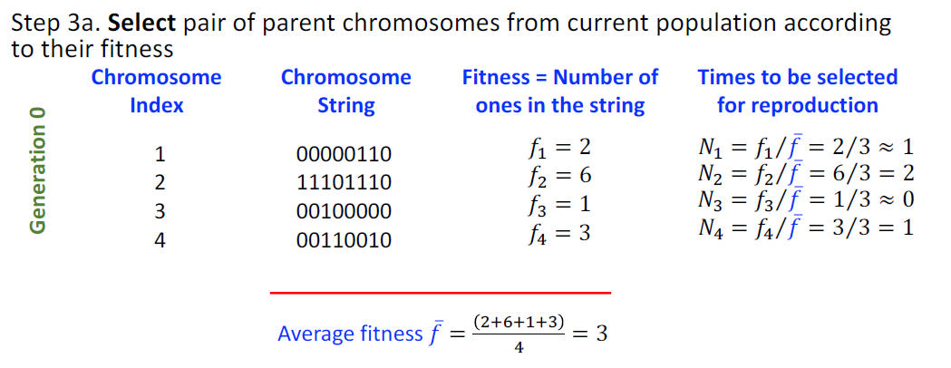
- Select pair of parent chromosomes from current population according to their fitness, i.e. chromosomes with higher fitness are selected more often.
- Apply crossover (with probability).
- Apply mutation (with probability of occurrence) .
- Apply generational replacement.
- Go to 2 or terminate if termination condition is met.
L25
Schema
A schema is a similarity template describing a subset of strings with similarities at certain string positions.
- Other name for a schema is a building block of a chromosome.
The Order of a schema 𝐻 is represented as 𝑂(𝐻) , denoting the number of defining symbols (non-* symbols) it contains.
The defining length of a schema 𝐻 is represented as 𝛿(𝐻) , denoting the maximum distance between two defining symbols.
Schema Theorem
Highly fit, short defining length, low order schemas increase exponentially in frequency in successive generations.

L26
Schema Theorem
Consider a specific schema 𝐻. If we use a classical GA with Roulette Wheel Selection, crossover (pc) and mutation (pm). We have: \[ m(H, t+1) \geq m(H, t) \cdot \frac{f(H, t)}{\bar{f}}\left(1-p_c \frac{\delta(H)}{l-1}-O(H) \frac{p_m}{l}\right) \] • 𝑚(𝐻,𝑡) represents the number of chromosomes matching schema 𝐻 at generation 𝑡, • 𝑓(𝐻,𝑡) represents the mean fitness of chromosomes matching schema 𝐻 at generation 𝑡, • \(\bar{f}\) represents the mean fitness of individuals in the population at generation 𝑡, • \(p_c\) \(p_m\) represent the probability of crossover and mutation, respectively, • 𝑙 is the length of each chromosome.